Simple Linear Regression – (Celsius to Fahrenheit).
What Is Linear Regression?
Linear regression is an algorithm that provides a linear relationship between an independent variable and a dependent variable to predict the outcome of future events. It is a statistical method used in data science and machine learning for predictive analysis.
The independent variable is also the predictor or explanatory variable that remains unchanged due to the change in other variables. However, the dependent variable changes with fluctuations in the independent variable. The regression model predicts the value of the dependent variable, which is the response or outcome variable being analyzed or studied.
Thus, linear regression is a supervised learning algorithm that simulates a mathematical relationship between variables and makes predictions for continuous or numeric variables such as sales, salary, age, product price, etc.
This analysis method is advantageous when at least two variables are available in the data, as observed in stock market forecasting, portfolio management, scientific analysis, etc.
A sloped straight line represents the linear regression model.
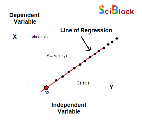
In the above figure,
X-axis = Independent variable
Y-axis = Output / dependent variable
Line of regression = Best fit line for a model
Here, a line is plotted for the given data points that suitably fit all the issues. Hence, it is called the ‘best fit line.’ The goal of the linear regression algorithm is to find this best fit line seen in the above figure.
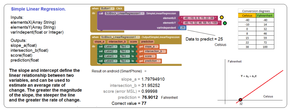
Using the regression extension, in the case of the line regression option, we will perform the temperature conversion calculation from Celsius to Fareheit. To ask for a data to be inferred we use the «VarIndependent» option.
Key benefits of linear regression.
Linear regression is a popular statistical tool used in data science, thanks to the several benefits it offers, such as:
.
- Easy implementation
The linear regression model is computationally simple to implement as it does not demand a lot of engineering overheads, neither before the model launch nor during its maintenance. - Interpretability
Unlike other deep learning models (neural networks), linear regression is relatively straightforward. As a result, this algorithm stands ahead of black-box models that fall short in justifying which input variable causes the output variable to change. - Scalability
Linear regression is not computationally heavy and, therefore, fits well in cases where scaling is essential. For example, the model can scale well regarding increased data volume (big data). - Optimal for online settings
The ease of computation of these algorithms allows them to be used in online settings. The model can be trained and retrained with each new example to generate predictions in real-time, unlike the neural networks or support vector machines that are computationally heavy and require plenty of computing resources and substantial waiting time to retrain on a new dataset. All these factors make such compute-intensive models expensive and unsuitable for real-time applications.
The above features highlight why linear regression is a popular model to solve real-life machine learning problems.
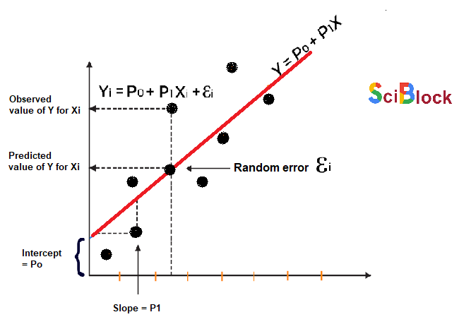
The regression model defines a linear function between the X and Y variables that best showcases the relationship between the two. It is represented by the slant line seen in the above figure, where the objective is to determine an optimal ‘regression line’ that best fits all the individual data points.
Mathematically these slant lines follow the following equation,
Y = m*X + b
Where X = dependent variable (target)
Y = independent variable
m = slope of the line (slope is defined as the ‘rise’ over the ‘run’)
However, machine learningOpens a new window experts have a different notation to the above slope-line equation,
y(x) = p0 + p1 * x
where,
y = output variable. Variable y represents the continuous value that the model tries to predict.
x = input variable. In machine learning, x is the feature, while it is termed the independent variable in statistics. Variable x represents the input information provided to the model at any given time.
p0 = y-axis intercept (or the bias term).
p1 = the regression coefficient or scale factor. In classical statistics, p1 is the equivalent of the slope of the best-fit straight line of the linear regression model.
pi = weights (in general).
Thus, regression modeling is all about finding the values for the unknown parameters of the equation, i.e., values for p0 and p1 (weights).
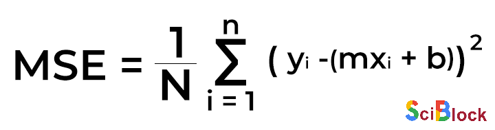
Furthermore, along with the prediction function, the regression model uses a cost function to optimize the weights (pi). The cost function of linear regression is the root mean squared error or mean squared error (MSE).
Fundamentally, MSE measures the average squared difference between the observation’s actual and predicted values. The output is the cost or score associated with the current set of weights and is generally a single number. The objective here is to minimize MSE to boost the accuracy of the regression model.
Math
Given the simple linear equation y=mx+b, we can calculate the MSE values:
Where,
N = total number of observations (data points)
1/N∑ni=1 = mean
yi = actual value of an observation
mxi+b = prediction
Along with the cost function, a ‘Gradient Descent’ algorithm is used to minimize MSE and find the best-fit line for a given training dataset in fewer iterations, thereby improving the overall efficiency of the regression model.
The equation for linear regression can be visualized as: