Neural Network – Music Classification.

Introduction.

Neural networks have found profound success in the area of pattern recognition. By repeatedly showing a neural network inputs classified into groups, the network can be trained to discern the criteria used to classify, and it can do so in a generalized manner allowing successful classification of new inputs not used during training. With the explosion of digital music in recent years due to Napster and the Internet, the application of pattern recognition technology to digital audio has become increasingly interesting.

Digital music is becoming more and more popular in people’s life. It is quite common for a person to own thousands of digital music pieces these days, and users may build their own music library through music management systems or software such as the Music Match Jukebox. However for professional music databases, labors are often hired to manually classify and index music assets according to predefined criteria; most users do not have the time or patience to browse through their personal music collections and manually index the music pieces one by one. On the other hand, if music assets are not properly classified, it may become a big headache when the user wants to search for a certain music piece among the thousands of pieces in a music collection. Manual classification methods cannot meet the development of digital music. Music classification is a pattern recognition problem which includes extraction features and establishing classifier. Many researchers have done a lot of works in this field and put forward some methods such as the rule-based audio classification method, the pattern match method, Hidden Markov Models (HMM), but they have own shortcomings, for example, rule-based audio classification can only be applied to identify the audio genres with simple characteristics, such as mute, so it is very difficult to meet the requirements of complex and multi-feature music. Pattern matching method needs to establish a standard mode for each audio type, so the calculation amount is large and classification accuracy is low. HMM method has poor classification decision ability and needs priori statistical knowledge.

Artificial neural network have found profound success in the area of pattern recognition, it can be trained to discern the criteria used to classify, and can do so in a generalized manner by repeatedly showing a neural network inputs classified into groups. Neural network provides a new solution for music classification, so a new music classification method is proposed based on BP neural network in this experiment.

Introduction to the problem.

We will use the Neural Network extension with the «MultiLayer with BackPorgation» module to train the neural network that uses the musical song data set. The dataset contains symbolic song features (MP3, in this case) and uses them to classify the recordings by genre. Each example is classified as a classical, rock, jazz or folk song. Furthermore, there will be different data sets depending on the characteristics that are adopted.

.
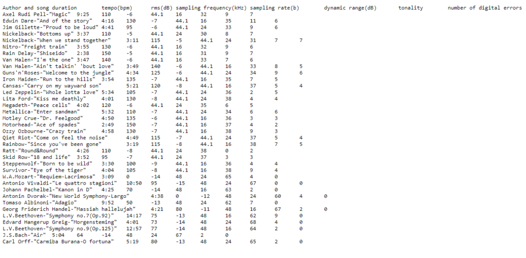
The attributes are song duration, tempo, root mean square (RMS) amplitude, sample rate, sample rate, dynamic range, tonality, and number of digital errors.
The main goal of this experiment is to train a neural network to classify these 4 gender types and find out which observed features have an impact on the classification.
The data set contains 100 instances (25 of each genre), 8 numerical attributes, and the name of the genre. Each instance has one of the 4 possible classes: classical, rock, jazz or folk.

Attribute Information:

Song’s duration in seconds
Tempo in beats per minute (BPM)
Root mean square (RMS) amplitude in dB. The RMS (Root-Mean-Square) value is the effective value of the total waveform. It is really the area under the curve. In audio it is the continuous or music power that the amplifier can deliver.
Sampling frequency in kHz
Sampling rate in b. There are two major common sample rate bases 44.1 kHz and 48 kHz. As most studio equipment uses recording and digital signal processing equipment working at a sample rate based on (a multiple of) 48 kHz the final result has to be re-sampled to the standard CD-format sample rate to be finally transferred onto a CD for distribution. This process includes losses and thus makes the audio signal on the CD slightly different (distorted) from the originally recorded signal. There are however other ways to distribute music in the format in which it was originally recorded and mastered. These formats are called studio master format.
A common frequency in computer sound cards is 48 kHz – many work at only this frequency, offering the use of other sample rates only through resampling. The earliest add-in cards ran at 22 kHz
Dynamic range(dr) in dB. Dynamic range, abbreviated DR or DNR, is the ratio between the largest and smallest possible values of a changeable quantity, such as in signals like sound and light. It is measured as a ratio, or as a base-10 (decibel) or base-2 (doublings, bits or stops) logarithmic value.
Tonality can be C, C#, D, D#, E, F, F#, G, G#, A, Bb and B, with associated values from 0 to 11 respectively.
Number of digital errors(nde) – There are two types of digital errors, glitches and clipping, but our number is sum of both, that is supplied using wavelab 7 software.
Glitches – These are disruptions in the audio. Glitches may occur after problematic digital transfers, after careless editing, etc. They manifest themselves as “clicks” or “pops” in the audio.
Clipping – A digital system has a finite number of levels that it can represent properly. When a sound has been recorded at too high a level or when digital processing has raised the level past what the system can handle, hard clipping occurs. This will be heard as a very harsh type of distortion.
Genre name: classic, rock, jazz and folk

Procedure of training a neural network.

In order to train a neural network, there are six steps to be made:

Normalize the data
Create a Neuroph project
Creating a Training Set
Create a neural network
Train the network
Test the network to make sure that it is trained properly

Step 1. Data Normalization.

In order to train neural network this data set have to be normalized. Normalization implies that all values from the data set should take values in the range from 0 to 1.
For that purpose it would be used the following formula or you can use module «Normalization Data» into extension Neural Network:

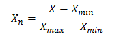
Where:

Where: X – value that should be normalized
Xn – normalized value
Xmin – minimum value of X
Xmax – maximum value of X

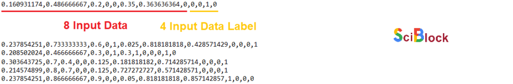
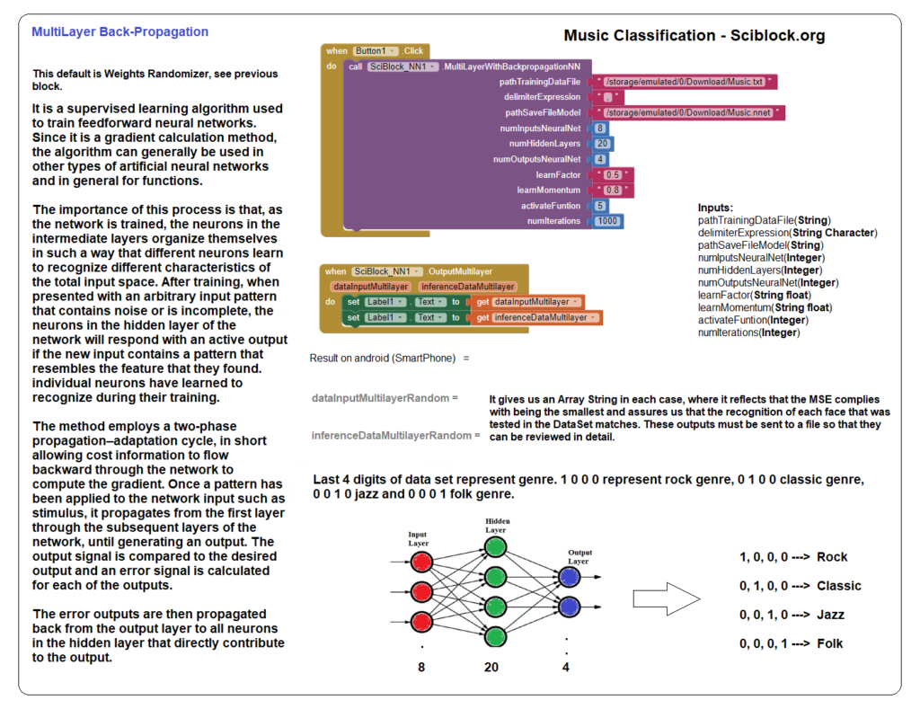
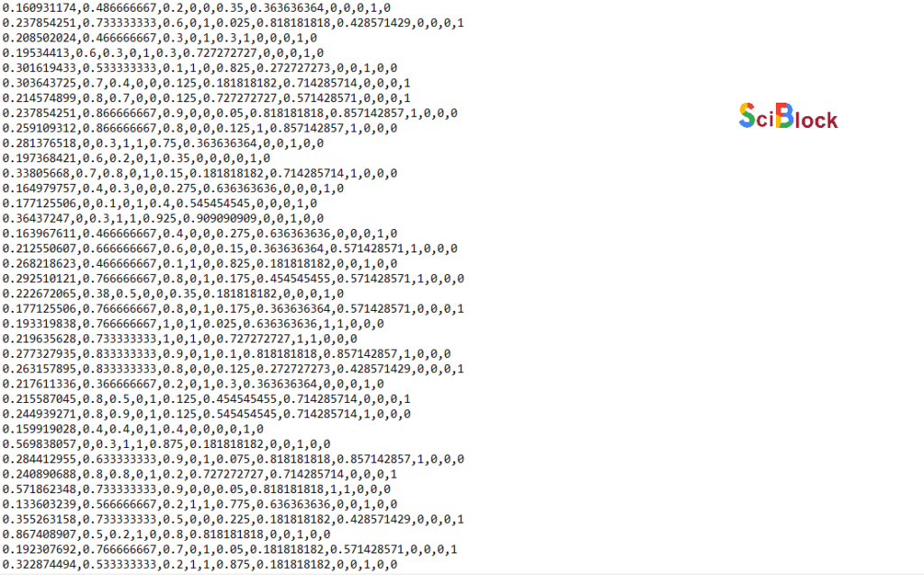
Last 4 digits of data set represent genre. 1 0 0 0 represent rock genre, 0 1 0 0 classic genre, 0 0 1 0 jazz and 0 0 0 1 folk genre.

Step 2, 3, 4, 5 (Using extension Neural Network).

Description of each parameter introduced in the model to train, execute and save. This model after saving it, which in this example will be named Music.nnet, can be used using the «ImportModelMultiLayer» module.

pathTrainingDataFile = This is the Path in the smartphone, where the DataSet is already normalized and ready to use in training.

delimiterExpression = In this example, the DataSet file with the name «Music.txt» has the data in each row separated or the delimiter is the comma character «,»

pathSaveFileModel = This is the Path in the smartphone, where the model after traning.

numInputsNeuralNet = Input data will be 8 from the DataSet for each row and 4 additional data, which are the labels that define the type of musical genre. The data inputs are the same number of input neurons. If we review the DataSet «Music.txt» in each row we will have 12 data that correspond to the total input data plus the sum of the 4 digits of the musical genre classification. We can see this more clearly below in the image where «Normalization DataSet» is specified.

numInputNeuralNet: Example of data in the dataset (normalized data), where the 8 entries and 4 labels are located for each row.

numHiddenLayers = Hidden layer layers where the MultiLayer BackPropagation algorithm is applied in this example. After applying several examples, we saw that one of the most appropriate quantities for this model is 20 layers, however this number will depend on each particular project.

numOutputsNeuralNet = The output neurons are directly proportional to the data that corresponds to the DataSet where the type of genre was labeled and corresponds to 4 output neurons. Le t us remember that the data to be inferred is the type of genre. Later we will see how we can infer data from test in the «ImportModelMultiLayer» module.

learnFactor = The learning rate is a tuning parameter in an optimization algorithm that determines the step size at each iteration while moving toward a minimum of a loss function.

learnMomentum = Momentum is a strategy for accelerating the convergence of the optimization process by including a momentum element in the update rule.

activate Funtion = An activation function determines if a neuron should be activated or not activated. This implies that it will use some simple mathematical operations to determine if the neuron’s input to the network is relevant or not relevant in the prediction process. There are different types of activation functions in our example we use SIGMOID.

numIterations = An iteration is a term used in machine learning and indicates the number of times the algorithm’s parameters are updated. The number of iterations will depend on when we reach the values most similar or equal to the data to be inferred in training. This can be calculated by comparing the training data with the inferred output data.

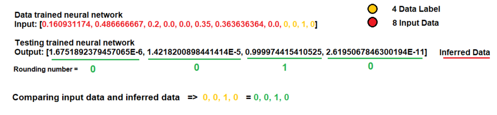
Example Training data (input) with inferred data (output) in our example gives us the following results after 1000 interactions.

Using Model MultiLayer Back-Propagation apply in Music Classification.

The most important point in creating any neural network model is the creation of the DataSet and its normalization. The dataset data must be well defined and carefully selected to represent the problem to be solved. (THIS POINT IS ONE OF THE MOST IMPORTANT IN THE CREATION OF THE MODEL).

DATASET EXAMPLE – MUSIC.TXT

NORMALIZATION DATASET – MUSIC.TXT

A segment of the training results, applying the model.

Using «ImportModelMultiLayer» extension module to infer test data.

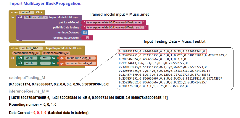
As we can see, the inferred data gives us correct data to be able to apply our model in practical cases.

Conclusions.

All models have been made on older devices (smartphones) with little processing power to ensure that current devices perform adequately in performance, for example this music rating example was a ZTE Blade L130 (2019) model. This model is very basic with 512 MB memory, 8GB storage, SPRD 4-core 1.3GHz CPU. The training was carried out on the same device and took approximately 29 seconds.

The above guarantees that any current or recent model’s performance will be optimal in final training and/or test execution.